¶ Introduction
The Duet 3 Expansion 1HCL ("closed-loop expansion board") provides a high current stepper motor driver that can be controlled in closed loop mode. This document provides a background in closed loop control (which may be skipped if the reader is already familiar with the concept) in addition to details on how to tune the closed loop system to operate optimally. For more details on the Duet 3 Expansion 1HCL, please see the 1HCL hardware overview page.
If you are just interested in the bare minimum required to get closed-loop functioning, skip ahead to the two 'What do I need to do?' sections below.
¶ Background on Closed Loop Control
A reader with prior knowledge of closed loop control may wish to skip the following sections on 'feedback' and 'PID controllers', however may still find the sections on 'closing the loop on stepper motors' and 'A Physical Interpretation of the 1HCL PID controller' beneficial.
¶ Feedback Control Systems
Control Theory concerns itself with controlling dynamical systems. A motor can be viewed as one such system if we simplify our understanding of a motor to a shaft that can have a torque applied to it to make it rotate, and that has some damping (such that a motor with no torque slows down over time). The job of a control system is to calculate how much torque is required, and when it should be applied, to move the motor to it's desired position.
Consider if you wanted to rotate the motor from 0 degrees to 90 degrees. You could apply just the right amount of torque so the motor speeds up, slows down, and lands exactly on 90 degrees. This method, however, would prove imprecise. It may not land on exactly 90 degrees, and any error introduced here would accumulate over more and more moves. This control system would be classified as 'open-loop' control.
A more precise system could use feedback of the motor's position to inform it's calculations. Imagine instead the system could sense how close it was to it's target. If it was far from it's target then it would apply a large torque, and as it got closer to it's target, it would apply less of a torque until eventually it was at it's target and applying zero torque. This type of control system, that uses feedback as a part of it's calculation, is classified as a 'closed-loop' system.
¶ PID Control Systems
One implementation of a closed loop controller is a PID controller. A 'controller' is simply a mathematical system that takes some set of inputs (including a target position), and outputs a control signal to make the system achieve the target position. In the case of a motor, the control signal is a 'torque' i.e. the controller can command the motor to produce some torque in order to reach the target position.
A PID controller has two inputs, the target and the feedback (current position). From this, the PID controller calculates the error as
error = target - feedback
It then also calculates the derivative and integral of that error with respect to time.
From these values, the control signal is then calculated as
control signal = Kd * error derivative + Kp * error + Ki * error integral
Where Kd, Kp and Ki are all constants of the user's choice.
The interactions between Kd, Kp and Ki are complex, but each can roughly be summarised as follows:
- Kp - How quickly the motor will reach it's target. However, moving fast may introduce overshoot and oscillations. A typical value may be 100-1000.
- Kd - Dampens down overshoot and oscillations. A typical value may be 0.01 - 0.1.
- Ki - Ensures the motor can maintain a stationary position under load. A typical value may be 100-1000.
A PID controller suffers from the limitation that when the load changes, the controller doesn't adjust the control signal until the increased load causes the error to increase. This effect can be mitigated by adding one or nomrew feedforward terms. In version 3.5 firmware the following feedforward terms are available:
- Kv - How much the control signal should be increased to allow for the additional load resulting from the motor angular velocity
- Ka - How much the control signal should be increased to allow for the extra load resulting from the motor angular acceleration
¶ A Physical Interpretation of the 1HCL PID controller
It is useful to have physical interpretations of the PID constants and control signal, as these can vary between controllers. Duet boards are implemented such that the following are true:
- Control Signal - Clamped between -256 and 256, where 256 represents the motor moving as fast as possible in the positive direction.
- Kp - A Kp of 1 with an error of 1 step will result in a control signal of 1
- Kd - A Kd of 1 with an error increasing at the rate of 1 step per second will result in a control signal of 1
- Ki - A Ki of 1 with an error of 1 step will result in a control signal of 1 after 1 second.
- Kv - a Kv of 1 will result in the control signal being increased by 1 if the motor speed is 1 full step per second
- Ka - a Ka of 1 will result in the control signal beibg increased by 1 if the motor acceleration is 1 full step per second per second
¶ Closing the Loop on Stepper Motors
As described above, a PID controller outputs a torque control signal. This means that our electronics must be able to induce this torque in the stepper motor, however this is not classically the way in which stepper motors operate. In order to understand how a torque can be applied, it is useful to revisit how a stepper motor works. A stepper motor has 2 coils that can have varying amounts of current running through them. Shown below left is a diagram of the current in these coils whilst the motor is taking four full steps. Each time the current changes, the shaft is pulled towards the next position. If we wanted to move more continuously instead of snapping, we could half each step (microstepping) - this is shown below middle. We can continue halving these steps as shown below right.
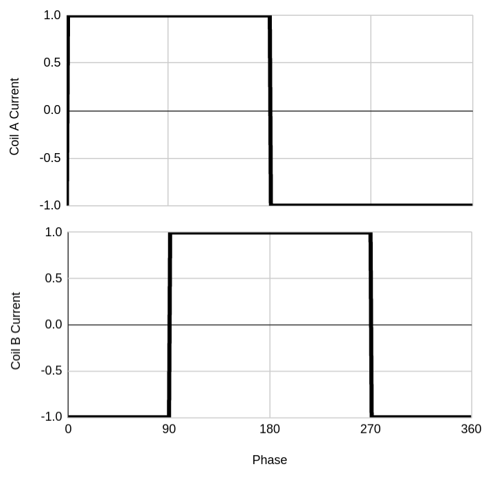
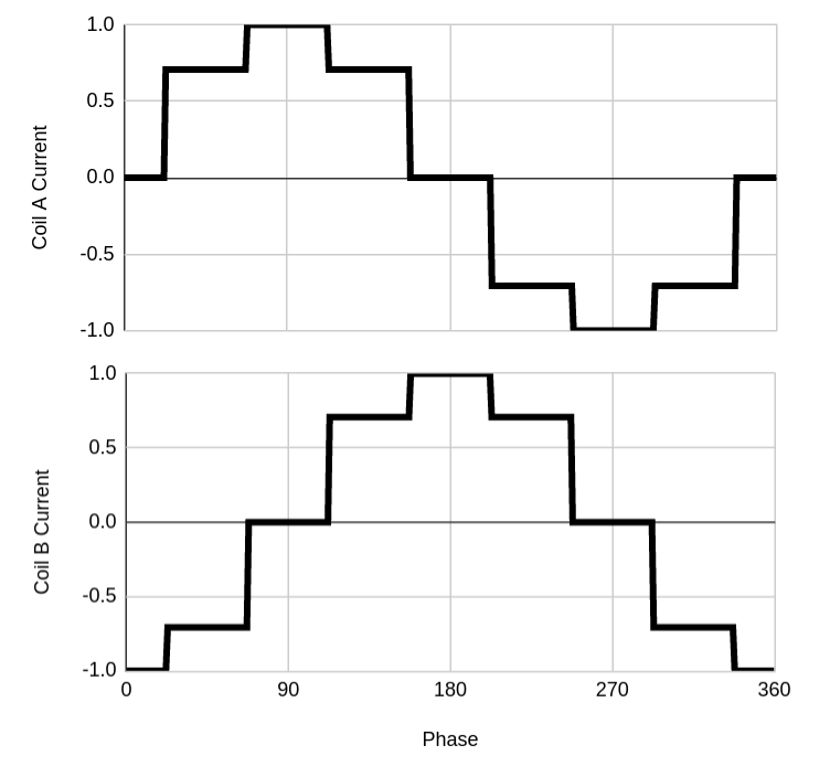
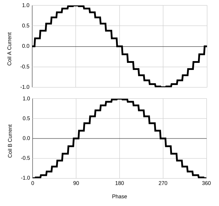
We can see that this approximates a sine and cosine wave. This means that if we applied a sine and cosine signal to the input coils, the motor would rotate continuously - i.e. experience a constant torque - let’s call this torque Tmax.
Therefore, to induce a torque of Tmax at any instance, we need to assert the value of sin(theta) on coil A and cos(theta) on coil B, where theta is representative of how far through a cycle of 4 steps the motor is. Intuitively, now that we know the current required to produce a torque of Tmax, we can find the current to produce a torque of a fraction of Tmax by multiplying the current by the fraction. Maximum torque is provided when the current through the coils is one full step ahead of the actual position of the rotor.
¶ Calibration and Tuning
The 1HCL closed loop driver requires the following:
- Calibration - Operations that must be performed before closed loop mode or assisted open loop mode (if supported) can be used
- PID Tuning - Adjusting the parameters of the PID control system to provide better response characteristics (e.g. reducing the steady-state error and preventing oscillation - see 'PID Control Systems' above)
¶ Calibration
As described above, the purpose of runtime tuning is to force the drive into a known state. Runtime tuning itself consists of a number of different manoeuvres, however the easiest to understand is the zeroing manoeuvre.
In order to perform a calibration operation, the M569.6 command is used. As per the GCODE dictionary, this command takes a driver address (P) and a manoeuvre number (V as in manoeuVre). The manoeuvre number of a quadrature shaft encoder calibration move is 1, so to run this manoeuvre on drive 0 of a 1HCL board at CAN address 50, one would run:
M569.6 P50.0 V1
Note that the drive must be in closed-loop or assisted-open-loop mode before this command can be run. See M569 D4 for putting a drive in one of these modes.
Running this command should make the drive move slightly: this quadrature tuning manoeuvre will at most make the motor move 6 full steps in each direction.
You will get a backlash for the motor reported, the backlash reading is a measure of how much stiction you have in your motor and the mechanics that constrain the rotation of the motor. The maximum allowed by the firmware is currently 0.22 full steps. The measured value typically reduces if motor current is increased.
Duet firmware currently only supports tuning one driver at a time. This means that when tuning a multi-driver axis, one driver will move and the other(s) will not. If attempting to tune a multi-driver axis, please take appropriate mitigation to ensure the axis doesn't become stressed/misaligned when only one one driver moves.
The table below lists the available calibration moves:
| Move ID | Move Name | Description | Required? | Movement performed | Time taken |
|---|---|---|---|---|---|
| 1 | Quadrature shaft encoder calibration | Detects in which orientation the stepper motor coils are connected and the phase relationship between the motor position and the encoder. This will also detect if a motor wiring is faulty or it is not plugged in. | For quadrature motor shaft encoders, this needs to be done after each power on or reset. Typically it is done as part of the homing file for the axis concerned. For linear composite encoders, this needs to be done just once when commissioning the system (the result is saved in the 1HCL flash memory). Not required for magnetic shaft encoders. | Quadrature shaft encoders: about 5 full steps forwards and then 5 back to original position. Linear composite encoders: about 20 full steps forwards and then 20 back to original position. | Quadrature shaft encoders: less than one second. Linear composite encoders: about four seconds. |
| 2 | Magnetic Encoder Calibration | Clears the encoder calibration, then calibrates the encoder positions to the motor. | For magnetic shaft encoders and linear composite encoders, this needs to be done just once for a combination of motor, encoder and 1HCL board. The results are stored in the 1HCL flash memory. Not required for quadrature shaft encoders. | For magnetic shaft encoders: just over one full motor revolution in each direction; for linear composite encoders: about five motor revolutions in each direction | Typically fifteen seconds to rotate the motor and capture the data, then ten seconds to process the data and store the calibration |
| 3 | Magnetic encoder calibration check | Checks that the encoder calibration is accurate and reports the residual error | Optional | As for magnetic encoder calibration | As for magnetic encoder calibration |
| 4 | Clear encoder calibration | Clears the encoder calibration. The encoder will need to be calibrated before the motor can be used in closed loop mode. This command can be used even when the driver is in open loop mode. | Run this if the motor or encoder that the 1HCL is connected to has changed, to prevent uncontrolled movements when the driver is switched into closed loop mode. | None | Less than one second |
¶ What do I Need to Do?
This depends on what type of encoder you are using. Read the appropriate section below and then advance to 'Running Tuning on Power On'.
¶ Quadrature Encoders
If you use a quadrature shaft encoder (i.e. your M569.1 command includes T2), then from the table above, manoeuvre 1 is required and it must be run every time the printer is powered on. This can be achieved by using the following command:
M569.6 P##.# V1 ; Where P##.# is the driver address to tune
Ideally this is put in the home#.g file for the axis that the motor is associated with. Until the motor has had this calibration move carried out, it will not move in closed loop mode. The normal procedure would be to home in open loop mode, then switch to closed loop mode or assisted open loop mode, then run the quadrature shaft encoder calibration move. See the Running Tuning on Power On section below.
¶ Magnetic Encoders (not supported before firmware 3.5)
If you use a magnetic encoder (i.e. your M569.1 command includes T3), then from the table above, manoeuvre 2 is required just once. The procedure for this is detailed in the 'Calibrating Magnetic Encoders' section below. Follow the instructions here, and then read the instructions in that section.
¶ Linear Composite Encoders (not supported before firmware 3.5)
If you are using a linear composite encoder (i.e. your M569.1 command includes T1), then from the table above, manoeuvre 2 and manoeuvre 1 are required just once. Perform manoeuvre 2 (magnetic encoder calibration) first.
¶ Running Quadrature Shaft Encoder Calibration at Power On
This is applicable to quadrature shaft encoders ony. The most suitable way to ensure tuning is run every time the printer is powered on is to modify the homing moves to include encoder calibration. This is because the motors make a small movement when they run the tuning move, and if the axis are homed before the move is made the printer can be in a known safe place to run the move.
A suitable new homing procedure is as follows:
- Home in open-loop mode
- Move to a known-safe position to perform tuning
- Switch to closed-loop mode or assited open loop mode
- Perform the quadrature shaft encoder calibration manoeuvre
- Move back to home
An example of this is shown below for a driver attached to the X axis, as driver 0 on the board at CAN address 50 with a quadrature shaft encoder:
; homex.g
; called to home the X axis

M569 P50.0 D0           ; Make sure we are in open loop mode

G91                     ; relative positioning
G1 H2 Z5 F6000          ; lift Z relative to current position
G1 H1 X-240 F3000       ; move quickly to X axis endstop and stop there (first pass)
G1 H2 X5 F6000          ; go back a few mm
G1 H1 X-240 F240        ; move slowly to X axis endstop once more (second pass)
G90                     ; absolute positioning

G1 X50 F3000            ; Move to a known-safe position
M400                    ; Wait for the move to complete
G4 P200                 ; Wait for the motor to settle
M569 P50.0 D4           ; Switch to closed loop mode
M569.6 P50.0 V1         ; Perform the calibration manoeuvre for a quadrature shaft encoder
G1 X0                   ; Move back to X0

G1 H2 Z0 F6000          ; lower Z again
Currently the RRF configuration tool will not generate these homing GCode files so they will need to be modified manually.
If tuning fails, the M569.6 command will report an error. In this case, check the troubleshooting section below.
¶ Calibrating Magnetic Encoders
Please read the following sections if you are using a magnetic encoder such as the Duet3D Magnetic Encoder.
Motivation
The magnetic sensor requires a magnet to be positioned on the back of the motor shaft. It is difficult to align the centre of the magnet precisely with the centre of rotation, so the calibration procedure measures how offset the magnet is and attempts to corrects for this in software. Since the magnet's position is not affected by cycling the printer's power, the calibration data is stored in non-volatile storage on the 1HCL, so that it only has to be run once. Note that if you replace the 1HCL, change the motor, move the encoder magnet, or remove the magnetic sensor board and re-attach it, you must re-run this calibration move.
Running the calibration procedure
To measure the offset, a little more than one full rotation of the motor is performed in each direction. Unlike other tuning moves, you can disconnect the motor from the axis - indeed, this is recommended because it reduces the load on the motor and makes calibration more accurate.
When you are satisfied that the motor can freely make up to 1.5 rotations in either direction, run the following command:
M569.6 P##.# V2 ; Where P##.# is the driver address to tune
Once this has been performed successfully, the values will be written to non-volatile memory on the 1HCL and remembered each time the power is cycled. The tuning can be re-run by simply running the M569.6 ... V2 command again, or checked by running the M569.6 ... V3 command.
The firmware will output the highest deviation of expected position vs encoder position recorded. This is useful as a proxy for how centered the magnet is.
¶ PID Tuning for closed loop mode
As discussed in the above 'PID Control Systems' section, the PID controller can be tuned by setting it's P, I and D parameters. Many methods exist for choosing parameters that lead to desirable characteristics for tuning PID loops in general. This is one example that is shown to work with the 1HCL boards with 48Ncm, 1.8degree, Nema 17 motors coupled with 1000ppr/4000cpr encoders.
Always run PID tuning with the motor current set to the highest value you intend to use. Increasing motor current after tuning the PID values may result in oscillation.
The tuning propcess described here is aimed at achieving maximum positioning accuracy (error between the commanded position and the motor position reduced as fast as possible). However, operating the motor in this way may be noisy because maximum current will be used to resolve small errors quickly. You may prefer to run with more relaxed PID settings to make the motor run more quietly, at the expense of a slightly greater lag between the commanded and actual position - but this lag may still be less than you would get in open loop mode. To do this, simply choose a lower P value (e.g. 30% or 50% of the value that gives the best rise time without oscillation), then tune the D and I values as normal.
¶ What do I need to do?
Possibly nothing! The 1HCL expansion board comes with PID parameters out of the box which may work sufficiently well for a basic use cases (P=100, I=0, D=0). However, the real power of closed-loop control comes when the PID controller is tuned for your specific setup. The sections below contain more details on how to tune your PID controller to achieve better results.
On average, tuning a PID controller results in an order of magnitude better performance, so whilst the factory default may work out of the box, tuning is very much recommended!
¶ Install the Closed Loop Plugin in Duet Web Control
In order to tune the PID controller manually, one needs to be able to visualise how the system is responding. To do this, use the closed loop plugin. First, download the 'closed-loop-plugin.zip' file from the assets section of the latest release. Once downloaded, upload the zip file (without decompressing) to your Duet by using System > Upload System Files, and follow the on-screen instructions to install the plugin. Finally, navigate to Setting > Machine Specific > Machine Specific Plugins and click the 'Start' button. For more details and troubleshooting, see the GitHub repository.
Once the plugin is installed & enabled, a new 'Closed Loop' item should appear on the left menu-bar (under Settings). Clicking into this will bring up the interface shown below.
This plugin is essentially a GUI for the M569.5 command - a command to record data from the closed loop system.
¶ Manual Tuning
- You must previously have run the required encoder calibration for the motor - see above.
- Use the M203 and M201 commands to set the maximum speed and acceleration of the axes concerned at least as high as you will ever want them to go
- Position the axis or axes to leave plenty of room for positive motion of the motor you want to tune. On a Cartesian machine you should normally start with the head close to the minimum X and Y values. On a CoreXY machine with the standard matrix, when tuning the X motor you should start near the minimum X and Y values, and when tuning the Y motor you should start close to minimum X and maximum Y.
- Make sure the motor is in closed loop mode
- Load the Closed Loop plugin and select Step Manoeuvre. A Step Manoeuvre Parameters panel should be shown. If it isn't then you have an old version of the Closed Loop plugin and you should download a later version.
- Start by setting the speed and acceleration parameters to modest values, and the movement length short (e.g. 25mm) in case you haven't set a suitable initial position
- In the plugin, select the driver you wish to tune
- In the Record panel select Current and Target Position, PID Control signal, and all five PID terms
- Select a modest P value e.g. 30. Set the I, D, A and V vales to zero
- Select 2000 samples collected at 2000 samples per second
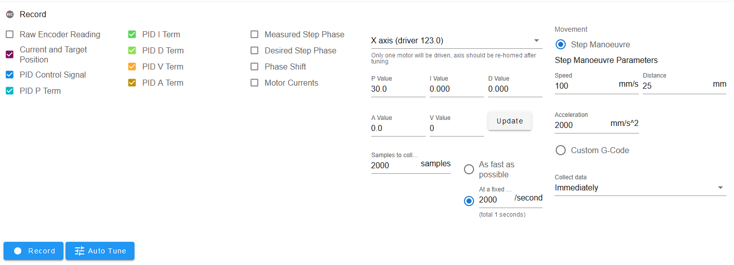
- Press Update to set the values
- Press Record to execute the movement and record the data. The motor will forwards by the specified amount and back again.
- (Note the 'Auto Tune' function has been removed from the closed loop plug-in v3.5.1 and later.)
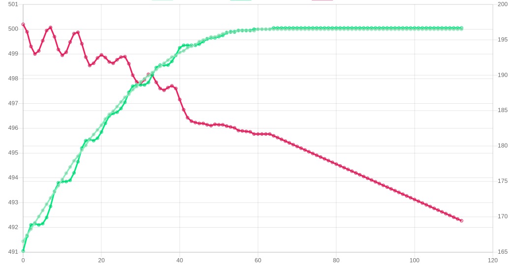
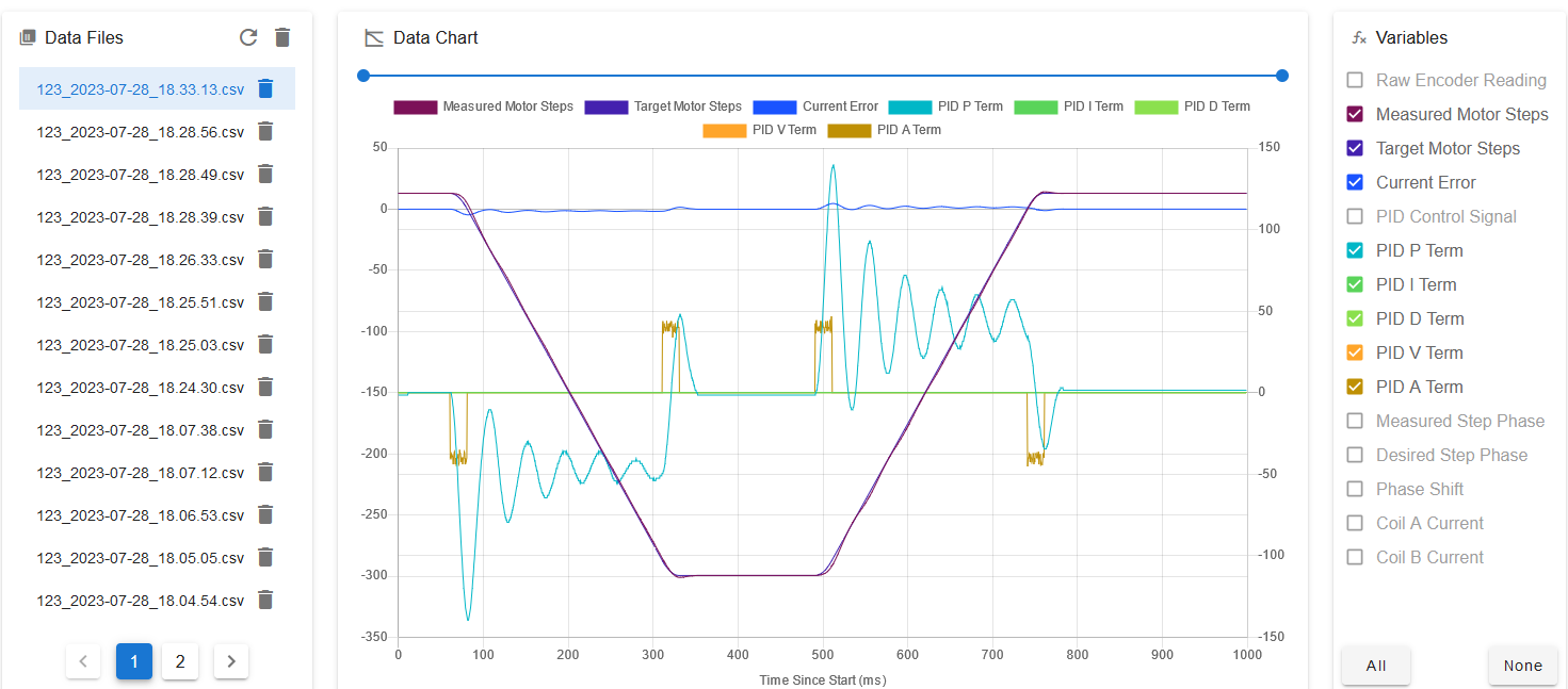
- Open the captured data file and select all available variables to plot except for the ID control signal. The plot should look something like this:
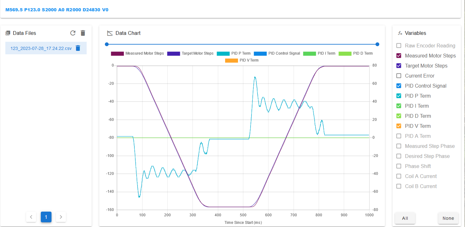
In this case there are modest damped oscillations in the PID P term dring the steady speed segments of the moves. If the oscillations are more severe, try reducing the P value.
Now you can try higher speeds and accelerations. You may need to increase the move length to make sure thet there is a steady speed section in each move. At ths stage, don't worry if you get some "Failed to maintain position" errors, because we haven't finished tuning yet. However, if you see any "Phase A short to ground" errors (and/or similar Phase B errors) then you will need to reset the driver. To do this use M18, then M17 to disable and re-enable it. Then select a lower maximum speed and try again.
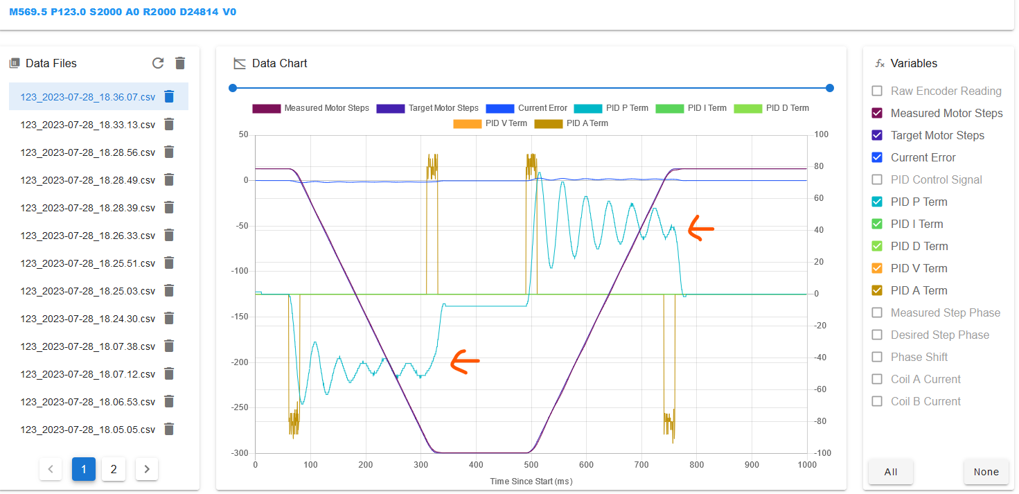
I ended up using speed 200mm/sec, acceleration 10000mm/sec^2, and move length 50mm (still with P=30 and all the other PID terms zero). The plot looked like this:
Notice that compared to the first plot, the peak PID P term has increased (note the change in axis scale on the right hand side).
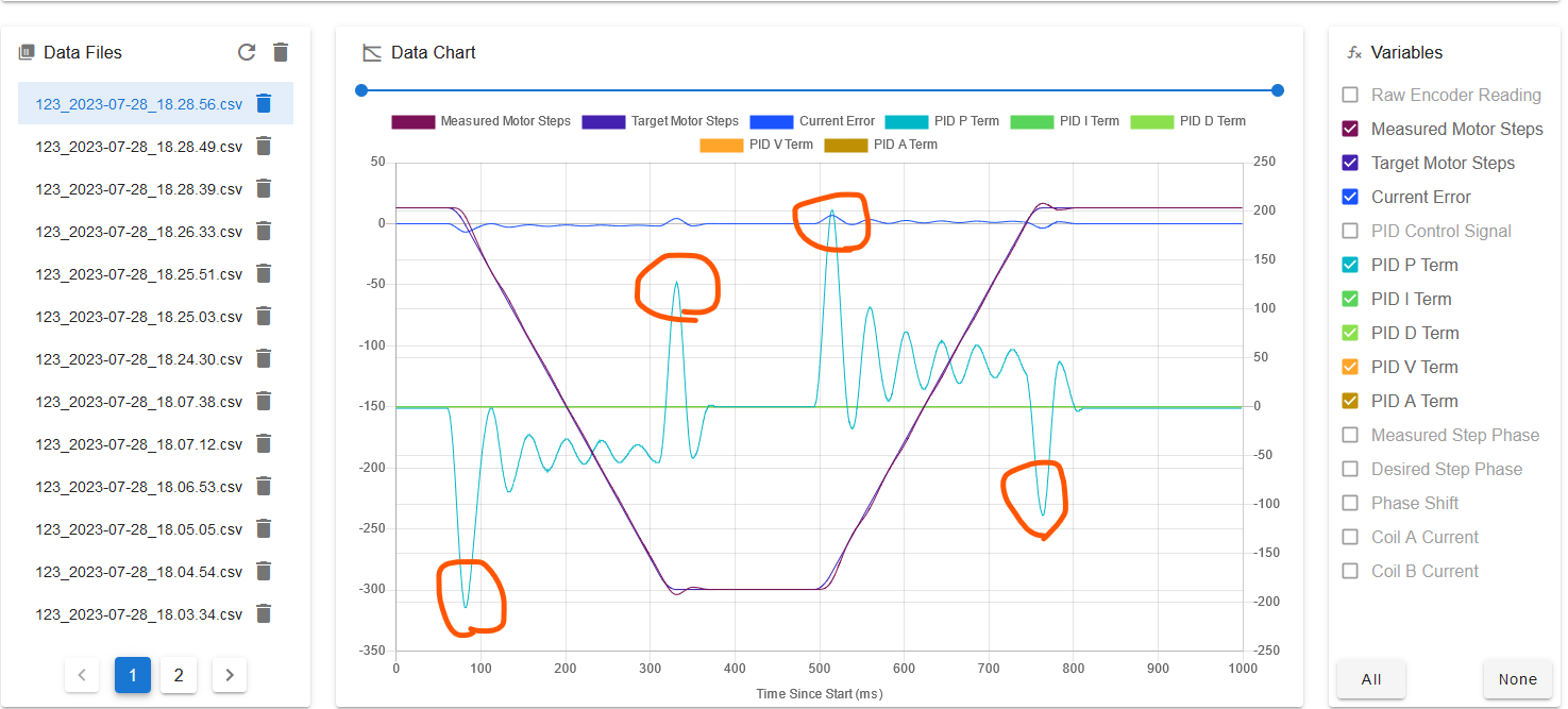
Now it's time to tune the A and V PID terms. First we want to tune the A term to eliminate the peaks in the PID P term during the acceleration and deceleration segments, which I have circled in orange in the above plot. Here's the same move but with the PID A term set to 100000:
The peaks in the P term have reduced from about 200 to less than 150 (note the change in scale on the right hand side again). Increasing the A term further to 200000 largely eliminated the peaks:
At the same time the "Failed to maintain position" errors went away.
Now that the A term is tuned we can tune the V term. The aim here is to reduce the average value of the PID P term during the steady speed segments, which I have indicated by the orange arrows in the previous plot. In this example a value of 400 gave me this plot, in which the average PID P term is close to zero:
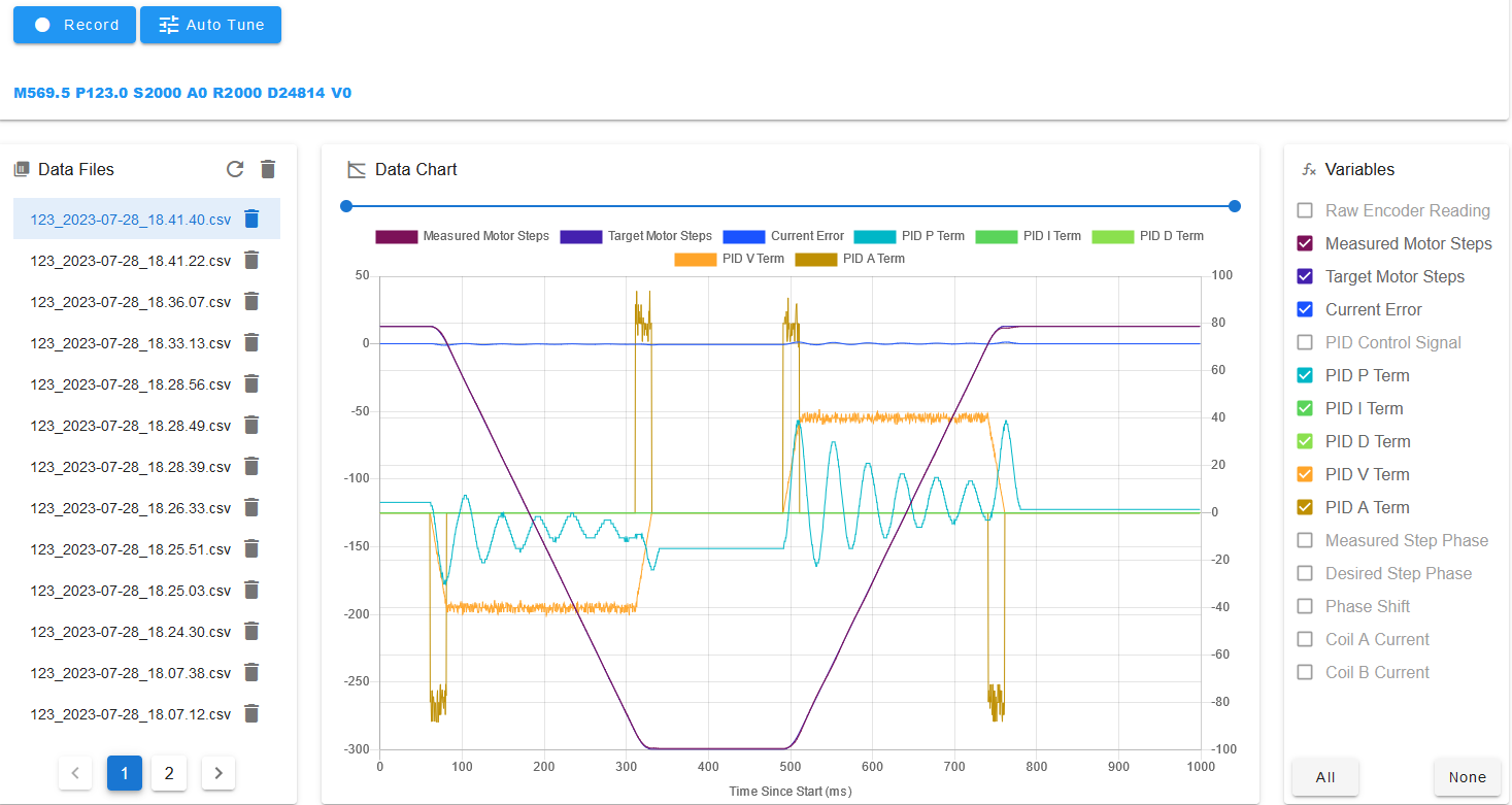
Next we want to reduce the amount of ripple on the P term. This can be done by using a nonzero D term. Setting the D term too high will make the motor sound raucous, so don't set it higher than necessary. I ended up with a value of 0.2 and this plot:
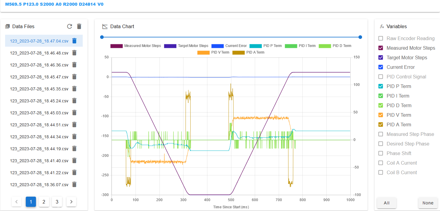
The remaining value to tune is the PID I parameter. This parameter is responsible for reducing the steady-state error to zero over a period of time. To see this error, turn off the display of all values except Current Error:
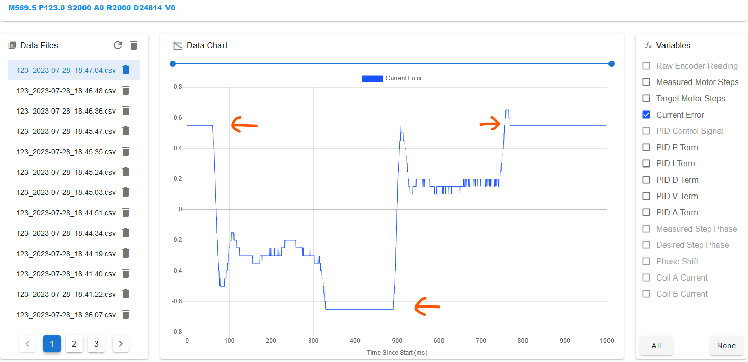
I have added orange arrows to highlight the error. Reduce it by adding a nonzero PID I parameter.
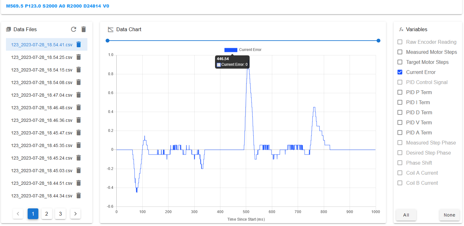
If you use too large a value for the I term, the position will oscillate. In this example, using an I term of 1000 reduce the error to zero in less than 100ms:
Now check the behaviour of the motor at a range of lower speeds. In this case I found that the motor noise was a little unpleasant at low speeds. I reduced the PID D term from 0.2 to 0.1 to make it more acceptable.
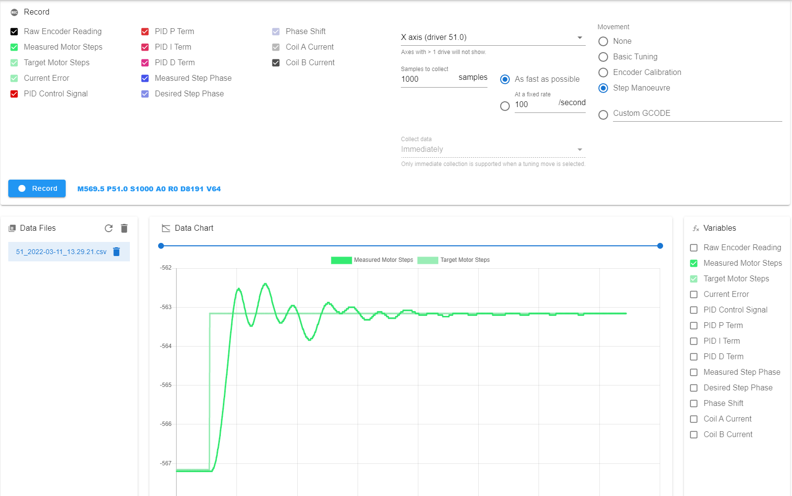
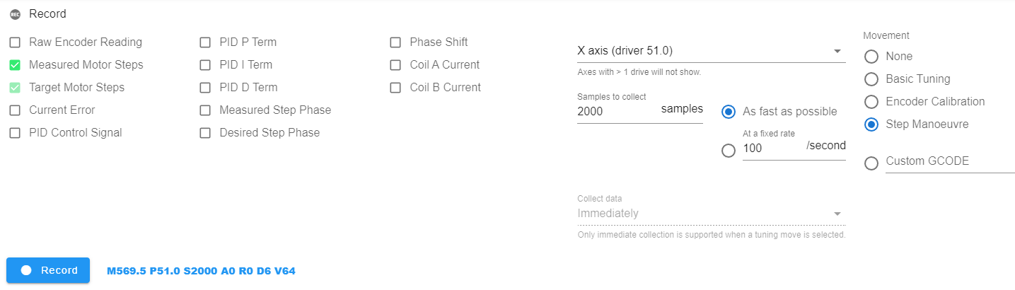
Use the plugin to execute the step manoeuvre. The settings shown below will record the response to a sidden change in desired position of 4 full steps. You must previously have run the required encoder calibration for the motor - see above.
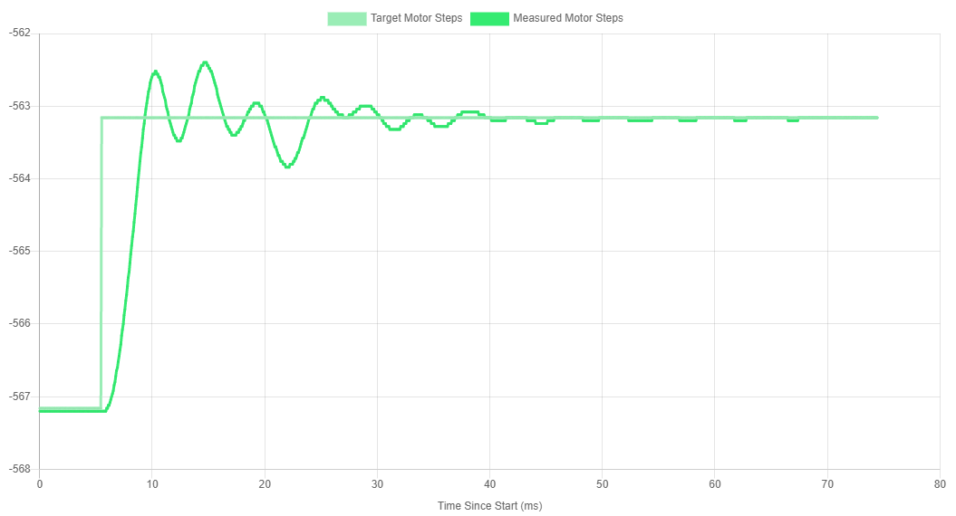
The following shows a typical response from the system - the black line represents the target, which steps up 4 steps at the start. The motor then reacts to meet this new target, at first overshooting and oscillating, and then settles down to roughly meet the target.
There are 3 features of interest in this graph, the rise time (how steep the initial rise is), the overshoot (how far the response exceeds the target) and the steady state error (how far above the target the response is after oscillations have settled)
In order to tune the PID system, we will adjust the tuning parameters, perform a step manoeuvre, and observe how the rise time, overshoot and steady state error change.
Warning: Incorrectly set PID parameters may cause unstable oscillations. This is where small oscillations grow larger exponentially. This may cause damage if the axis oscillates out of control. Always be ready to trigger an emergency stop. It is recommended that you first disconnect the motor from the axis in order to tune. This will not give precise tuning results, but will give you a feel of what can induce oscillations in your motor. Once you are comfortable with preventing oscillations, hook your motor back up to the drive.
To set up for tuning, set all gains to zero, and the holding current to 100:
M569.1 P##.# R0 I0 D0    ; Where P##.# is the address of the driver being tuned
M917 #100                ; Where # is the axis being tuned (X, Y or Z)
¶ Tuning P
First, gradually increase the value of the proportional constant (R) until the rise time does not improve noticeably.
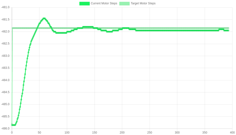
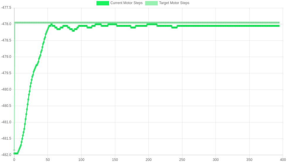
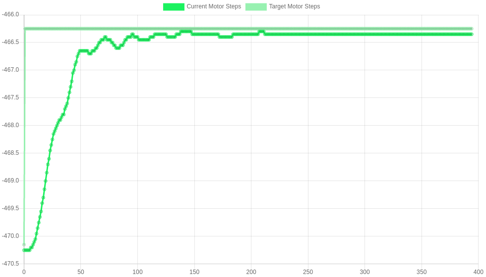
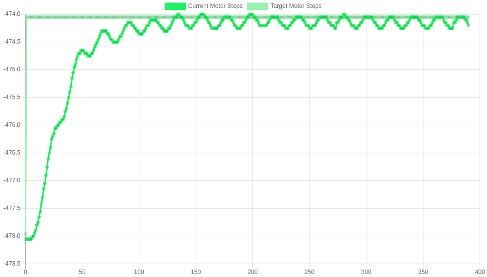
The images below show some responses for P=50, 75, 150 and 200 respectively. Improvements are seen up to P=150, but not in P=200. This gives a value for P of 150.
P=50 M569.1 P##.# R50 I0 D0 |
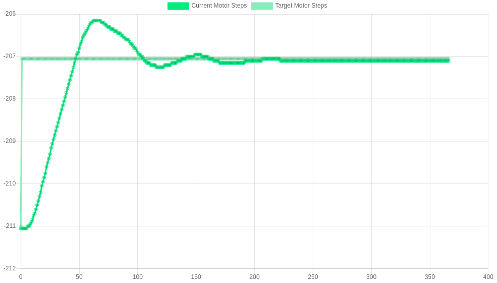 |
P=75 M569.1 P##.# R75 I0 D0 |
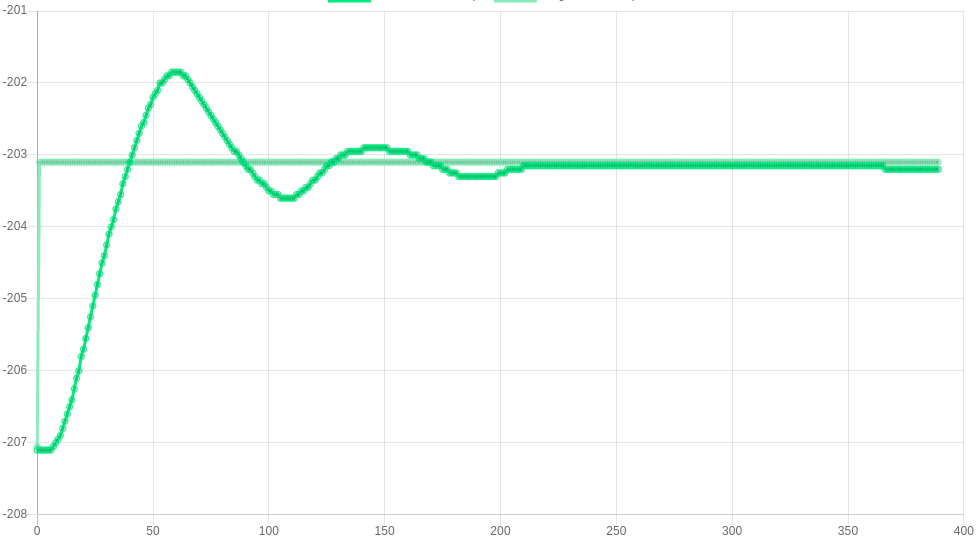 |
P=150 M569.1 P##.# R150 I0 D0 |
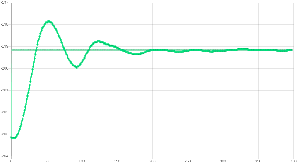 |
P=200 M569.1 P##.# R200 I0 D0 |
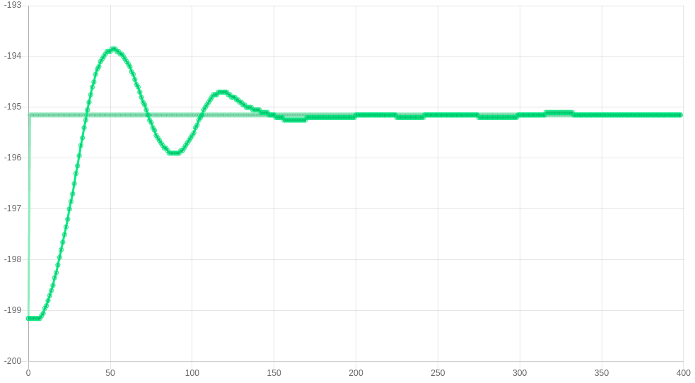 |
Note that tuning P in this way makes the motor as responsive as possible, at the expense of motor noise. You may prefer to select a lower value of P (see below) before tuning the other parameters.
¶ Tuning D
The next stage is to increase the derivative constant (D) until there is no overshoot (this is called being 'critically damped'). However, a large D term will start to introduce oscillations, so we want to use the lowest value of D that gets us critically damped. Exceedingly large D terms may cause runaway oscillations - so be careful!
The images below show some responses for D=0.1, 0.2, 0.25 and 0.3 respectively. The response becomes critically damped at 0.2, so D=0.2 is used. 0.3 shows an example of oscillations - this is what you want to avoid!
D=0.1 M569.1 P##.# R150 I0 D0.1 |
 |
D=0.2 M569.1 P##.# R150 I0 D0.2 |
 |
D=0.25 M569.1 P##.# R150 I0 D0.25 |
 |
D=0.3 M569.1 P##.# R150 I0 D0.3 |
 |
¶ Tuning I
The final parameter to adjust is the I parameter. This should be set to reduce the 'steady state' error to zero (the steady state error is the error seen once the response has settled down). The graphs above show 400 samples, when tuning the I parameter it can be useful to go higher. 1000 samples is usually enough to view the steady state response. In addition, it is useful to plot the 'current error' instead of 'target/current motor steps'.
The images below show some responses for I=0, 500, 5000 and 50,000 respectively. I=5000 shows the steady state being reduced to zero, so this would be a suitable choice here. I=50,000 shows an I term that is too large - large (unsafe) oscillations are introduced.
I=0 M569.1 P##.# R150 I0 D0.2 |
 |
I=500 M569.1 P##.# R150 I500 D0.2 |
 |
I=5000 M569.1 P##.# R150 I5000 D0.2 |
 |
I=50000 M569.1 P##.# R150 I50000 D0.2 |
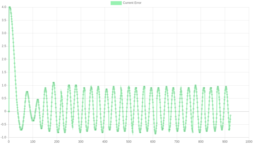 |
At the end of these steps a configuration of P=150, I=5000 and D=0.2 has been found. This was for the x-axis drive of an Ender 3, but these values will be different for your configuration. For example, one would expect a drive with a static load (such as a z-axis) to require a larger I term to account for this. Save your configuration to config.g by updating the M569.1 line to include these newfound tuning parameters.
¶ Testing the Tuning Parameters
In order to investigate how well the tuning has worked, a G1 move can be recorded. Below is a configuration that will record samples of a G1 move:
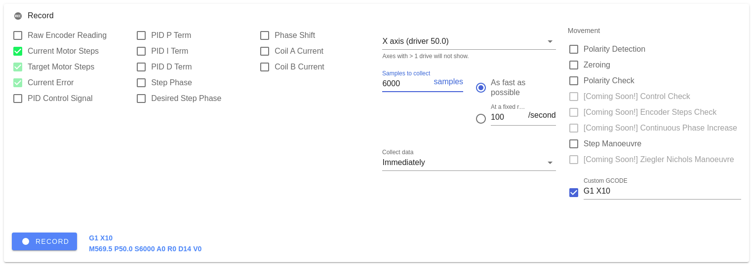
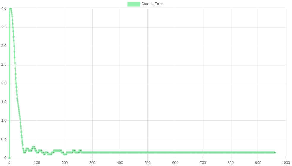
As an example, this is the result after using the above to tune an Ender 3 x-axis:
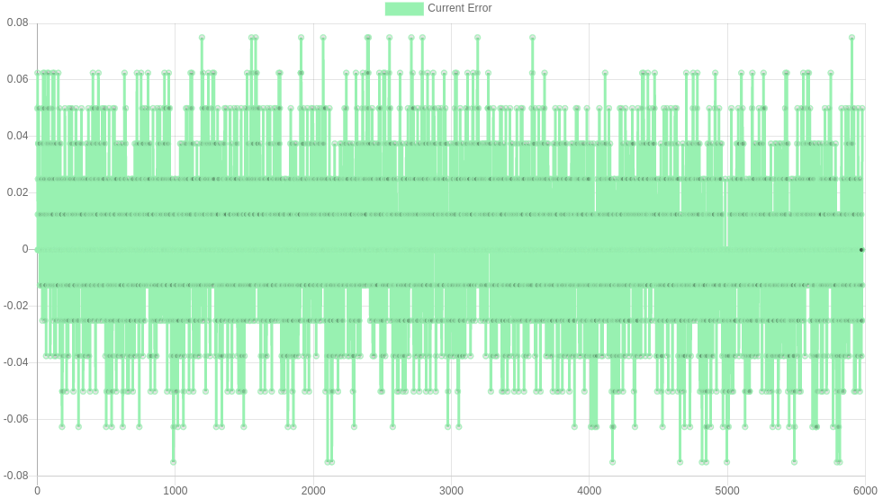
The maximum error here is only 0.08 of a step. The graph shows points only at ±4 discrete locations - this corresponds to the resolution of the encoder. It is harder to get better control when the error signal is hovering around the resolution of the encoder, so this drive has been successfully tuned.
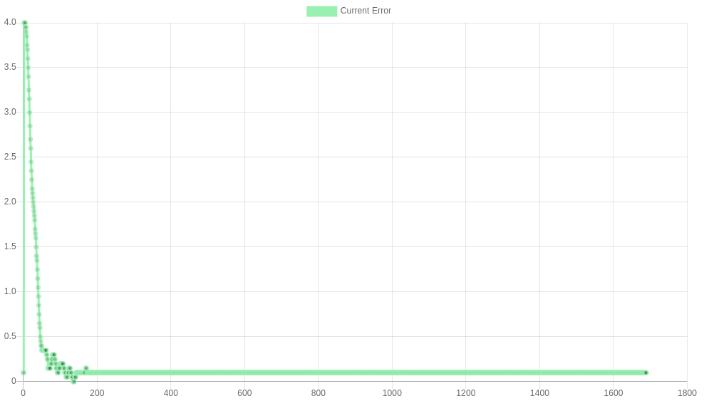
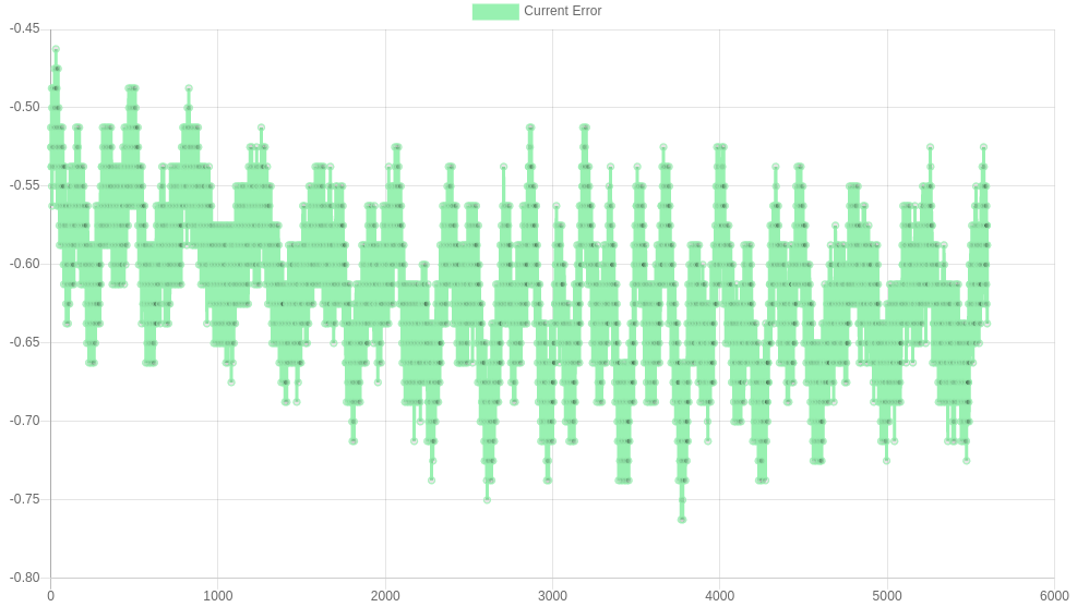
For comparison, below is the same graph, but for the factory default tuning parameters. The error is still below 1 step, however is an order of magnitude worse than what has been achieved by tuning. In addition, the tuned controller keeps the average error to zero, however the factory-default controller has an average error of over half a step!
¶ Noise reduction
You might have noticed that your motor makes a noise similar to white noise after tuning. The reasons for this can be seen by plotting the PID control signal and it's components on a G1 move:
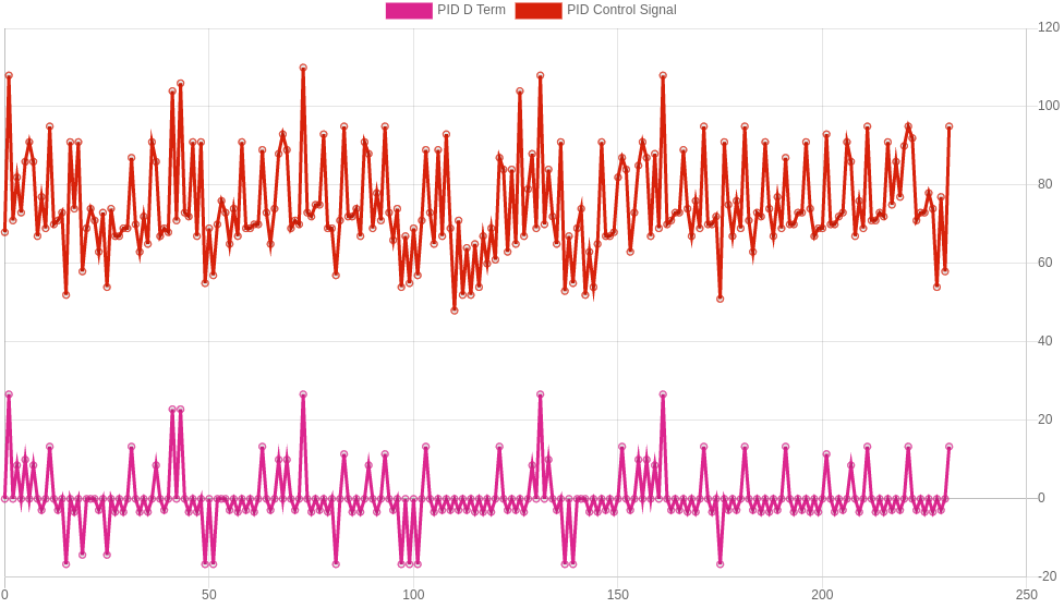
The PID signal has a large portion of noise introduced by the D term. This isn't too much of a surprise since even small amounts of noise will be picked up by the D term as large gradients, and amplified.
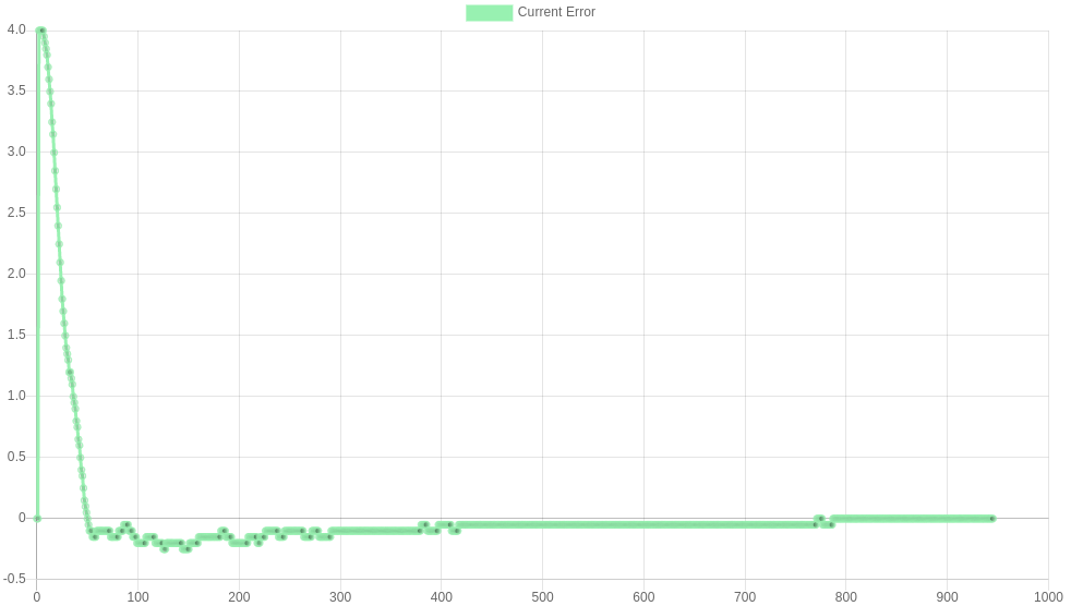
In order to reduce this noise, the D term can be set to zero, however this will increase overshoot and therefore have an effect on accuracy. When a G1 command is run on the Ender 3 example above, a tuned D value gives a maximum error of ± 0.07 steps. When using D=0, that error is increased to ± 0.1 steps, however the motor runs much quieter. This is still an order of magnitude better than the factory-default parameters.
A better way to reduce noise is to accept a slightly worse step response by reducing the P term. This in turn will reduce the optimum D term, which will reduce the noise.
It is a matter of personal preference weighing up the sound of the motors against the decreased accuracy.
¶ Setting parameters for Assisted Open Loop mode in RRF 3.5 and later
If you wish to use Assisted Open Loop mode instead of Closed Loop mode then tuning is much simpler:
- The PID P term should be set to 200. You should not need to change it.
- The PID I term is not used.
- The PID D term can typically be set to zero.
- The A and V terms will not affect the PID P term, so you can't tune them in the same way. However, you may be able to achieve slightly higher speeds and/or accelerations by using nonzero A and/or V terms.
¶ Reporting failure to maintain position
If you want failure to maintain the desired position to be reported, you must use the E parameter of the M569.1 command to set a suitable error threshold. This must obviously be higher than the maximum error that you get in mormal use. Therefore you will first need to run PID tuning so as to minimise the position errors, then you can take the highest residual error reported by the input shaping plugin and use an error threshold somewhat greater than that.
With the M569.1 E parameter correctly specified, failure to maintain position will be reported via the event system.
¶ Troubleshooting
¶ Error on M569.6 tuning/calibration command
Error: M569.6: Driver 20.0 basic tuning failed, the measured motion was inconsistent
This message means either that there was an issue with the encoder or that the motor did not move smoothly.
- Check the encoder wiring.
- If you're using the single-ended quadrature connection, make sure to put a jumper on "quadrature differential/single ended select".
- If you're using the differential quadrature connection, make sure to remove any jumper on "quadrature differential/single ended select".
- Increase the motor current.
- If the motors are already connected to the motion system by belts, try removing the belts to see if tuning can then be accomplished.
Error: M569.6: Driver 20.0 basic tuning failed, the measured motion was less than expected, measured counts/rev is about 1014.2 or the measured motion was more than expected
This message means that the expected encoder pulses per revolution (PPR) set by M569.1 C parameter was not what was measured. Check the specification of the encoder; 1000PPR is fairly standard. Usually you can change the M569.1 C parameter to close to what is suggested by the firmware.